Understanding the Basics of Markdown

Writing

Markdown

Documentation

Author

Tako

Published

December 14, 2025

NumPyroを使ってベイズ回帰モデルの実装

参照させていただいた記事: 【ベイズ統計モデリング入門】NumPyroで回帰モデルをつくる

Code

import pandas as pd
import matplotlib.pyplot as plt
import seaborn as sns

import jax.numpy as jnp
from jax import random, vmap, grad, jit, lax

import numpyro
from numpyro import plate, sample
from numpyro.infer import MCMC, NUTS, Predictive
import numpyro.distributions as dist

Code

# チップのデータセット
df = sns.load_dataset("tips")

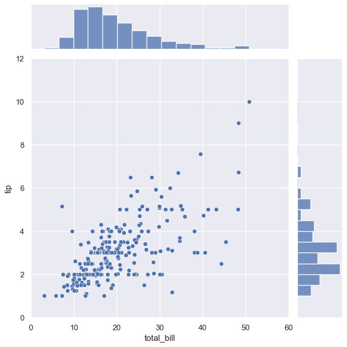
# 会計総額とチップのデータを可視化
sns.set(style="darkgrid")
sns.jointplot(
    x="total_bill",
    y="tip",
    data=df,
    kind="scatter",
    xlim=(0, 60),
    ylim=(0, 12),
    color="b",
    height=7,
)

Code

df.head()

	total_bill	tip	sex	smoker	day	time	size
0	16.99	1.01	Female	No	Sun	Dinner	2
1	10.34	1.66	Male	No	Sun	Dinner	3
2	21.01	3.50	Male	No	Sun	Dinner	3
3	23.68	3.31	Male	No	Sun	Dinner	2
4	24.59	3.61	Female	No	Sun	Dinner	4

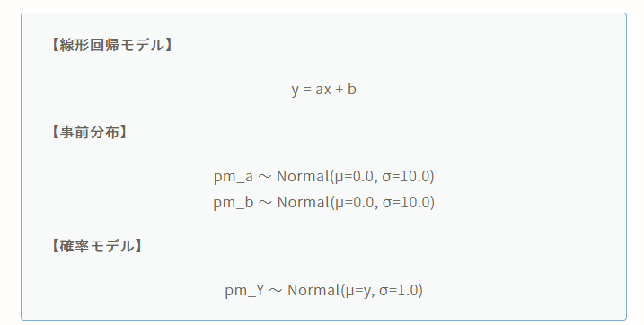
-線形回帰モデル-

Code

# 線形回帰モデルの設計
def model(X, Y=None):
    pm_a = numpyro.sample("pm_a", dist.Normal(0, 10))
    pm_b = numpyro.sample("pm_b", dist.Normal(0, 10))

    mu = pm_a * X + pm_b
    sigma = 1.0

    pm_Y = numpyro.sample("pm_Y", dist.Normal(mu, sigma), obs=Y)

    return pm_Y

MCMCの実行

Code

# dfからnumpy.ndarrayに変換
Y = df["tip"].values  # 目的変数：Y = [y0, y1, y2, ... yi]
X = df["total_bill"].values  # 説明変数：X = [x0, x1, x2, ... xi]

Code

# RUN MCMC
# NUTS (No-U-Turn Sampler) is an adaptive variant of the Hamiltonian Monte Carlo (HMC) algorithm
# HMCのステップサイズや反復回数などのパラメータを自動調整
# 効率的なサンプル
# 収束の改善
# https://qiita.com/dai08srhg/items/5d4ac3070bae836aef10
kernel = NUTS(model)
mcmc = MCMC(kernel, num_warmup=1000, num_samples=2000)
mcmc.run(rng_key=random.PRNGKey(0), X=X, Y=Y)

# print MCMC summary（推定パラメータの基本統計量）
mcmc.print_summary()

sample: 100%|██████████| 3000/3000 [00:00<00:00, 3616.90it/s, 11 steps of size 2.54e-01. acc. prob=0.94]


                mean       std    median      5.0%     95.0%     n_eff     r_hat
      pm_a      0.11      0.01      0.11      0.09      0.12    368.76      1.00
      pm_b      0.90      0.16      0.90      0.65      1.17    377.02      1.00

Number of divergences: 0

Code

# get param (num_samples=2000)
mcmc_samples = mcmc.get_samples()
pm_a = mcmc_samples["pm_a"]
pm_b = mcmc_samples["pm_b"]

print("mcmc_samples:", mcmc_samples)
print("pm_a:", pm_a)
print("pm_b:", pm_b)

mcmc_samples: {'pm_a': Array([0.10649762, 0.110033  , 0.10530762, ..., 0.11129791, 0.10644959,
       0.10579225], dtype=float32), 'pm_b': Array([0.86267745, 0.9398046 , 0.9131396 , ..., 0.751051  , 0.8998211 ,
       0.8538504 ], dtype=float32)}
pm_a: [0.10649762 0.110033   0.10530762 ... 0.11129791 0.10644959 0.10579225]
pm_b: [0.86267745 0.9398046  0.9131396  ... 0.751051   0.8998211  0.8538504 ]

Code

len(set(pm_a.tolist()))

Code

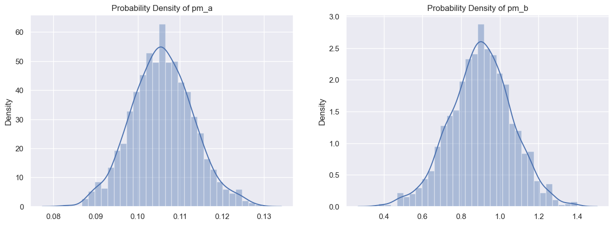
# 可視化
sns.set(style="darkgrid")
plt.figure(figsize=(15, 5))
plt.subplot(1, 2, 1)
sns.distplot(pm_a)
plt.title("Probability Density of pm_a")

plt.subplot(1, 2, 2)
sns.distplot(pm_b)
plt.title("Probability Density of pm_b")
plt.show()

C:\Users\takuk\AppData\Local\Temp\ipykernel_27764\3318693772.py:5: UserWarning: 

`distplot` is a deprecated function and will be removed in seaborn v0.14.0.

Please adapt your code to use either `displot` (a figure-level function with
similar flexibility) or `histplot` (an axes-level function for histograms).

For a guide to updating your code to use the new functions, please see
https://gist.github.com/mwaskom/de44147ed2974457ad6372750bbe5751

  sns.distplot(pm_a)
C:\Users\takuk\AppData\Local\Temp\ipykernel_27764\3318693772.py:9: UserWarning: 

`distplot` is a deprecated function and will be removed in seaborn v0.14.0.

Please adapt your code to use either `displot` (a figure-level function with
similar flexibility) or `histplot` (an axes-level function for histograms).

For a guide to updating your code to use the new functions, please see
https://gist.github.com/mwaskom/de44147ed2974457ad6372750bbe5751

  sns.distplot(pm_b)

Code

X_range = jnp.linspace(0, 50, 51)

predictive = Predictive(model, mcmc_samples)
predict_samples = predictive(random.PRNGKey(1), X=X_range, Y=None)
print(predict_samples)

{'pm_Y': Array([[ 1.810429  ,  0.02438818,  0.22200845, ...,  5.2724934 ,
         6.715812  ,  6.422859  ],
       [ 0.15076251,  0.8095171 ,  0.21540537, ...,  5.2437186 ,
         7.817451  ,  6.173345  ],
       [ 2.476837  ,  0.21040367,  0.42815638, ...,  8.04783   ,
         7.40407   ,  5.8891115 ],
       ...,
       [ 1.0230944 ,  1.1552314 ,  0.25326768, ...,  4.831621  ,
         7.0255423 ,  5.759563  ],
       [ 1.5060548 , -0.62601656,  1.4508446 , ...,  5.9778643 ,
         6.058488  ,  4.774219  ],
       [ 1.0496006 ,  0.51519567,  1.4674567 , ...,  5.349556  ,
         4.992259  ,  6.651703  ]], dtype=float32)}

Code

pm_Y = predict_samples["pm_Y"]
print(pm_Y)

[[ 1.810429    0.02438818  0.22200845 ...  5.2724934   6.715812
   6.422859  ]
 [ 0.15076251  0.8095171   0.21540537 ...  5.2437186   7.817451
   6.173345  ]
 [ 2.476837    0.21040367  0.42815638 ...  8.04783     7.40407
   5.8891115 ]
 ...
 [ 1.0230944   1.1552314   0.25326768 ...  4.831621    7.0255423
   5.759563  ]
 [ 1.5060548  -0.62601656  1.4508446  ...  5.9778643   6.058488
   4.774219  ]
 [ 1.0496006   0.51519567  1.4674567  ...  5.349556    4.992259
   6.651703  ]]

Code

len(pm_Y)

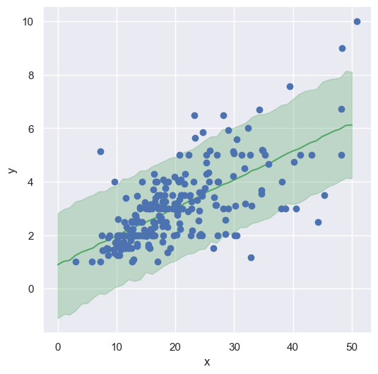
推論

Code

mean_Y = pm_Y.mean(axis=0)
y_low, y_high = jnp.percentile(pm_Y, jnp.array([2.5, 97.5]), axis=0)

# 可視化
fig = plt.figure(figsize=(6.0, 6.0))
plt.plot(X_range, mean_Y, "-", color="g")
plt.fill_between(X_range, y_low, y_high, color="g", alpha=0.3)
plt.plot(X, Y, "o")
plt.xlabel("x"), plt.ylabel("y")
plt.show()

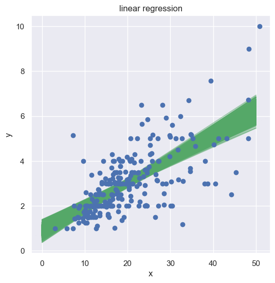
全てのパラメターを使って推論

Code

N = len(pm_a)
# X_range = jnp.linspace(0, 50, 50)

# 予測結果の可視化
fig = plt.figure(figsize=(6.0, 6.0))
for i in range(N):
    pm_y = [pm_a[i] * x + pm_b[i] for x in X_range]
    plt.plot(X_range, pm_y, "g-", alpha=0.5)

# データセットの可視化
plt.plot(X, Y, "o")
plt.xlabel("x"), plt.ylabel("y")
plt.title("linear regression")
plt.show()

Code

def my_model(mcmc_samples, X):
    """線形回帰モデル"""
    mcmc_samples = mcmc.get_samples()
    pm_a = mcmc_samples["pm_a"]
    pm_b = mcmc_samples["pm_b"]

    # 平均値
    mu_a = jnp.mean(pm_a, axis=0)
    mu_b = jnp.mean(pm_b, axis=0)
    print("mu_a=", mu_a)
    print("mu_b=", mu_b)

    # 線形回帰モデル
    Y_hat = mu_a * X + mu_b

    return Y_hat

Code

# 予測値
Y_hat = my_model(mcmc_samples, X)

# 可視化
fig = plt.figure(figsize=(6.0, 6.0))
plt.plot(X, Y, "o")
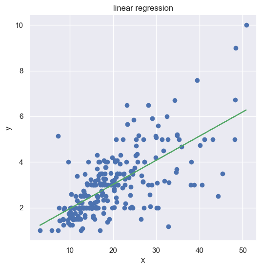
plt.plot(X, Y_hat, "g-")
plt.xlabel("x"), plt.ylabel("y")
plt.title("linear regression")
plt.show()

mu_a= 0.10581156
mu_b= 0.9027909

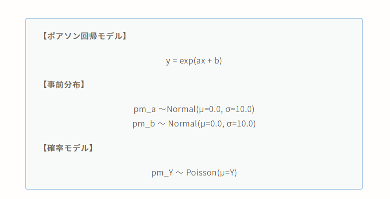
ポアソン回帰モデル

Code

# ポアソン回帰モデルの設計
def model(X, Y=None):
    pm_a = numpyro.sample("pm_a", dist.Normal(0.0, 10.0))
    pm_b = numpyro.sample("pm_b", dist.Normal(0.0, 10.0))

    theta = pm_a * X + pm_b
    mu = jnp.exp(theta)

    numpyro.sample("pm_Y", dist.Poisson(mu), obs=Y)

Code

# Run MCMC
kernel = NUTS(model)
# mcmc = MCMC(kernel, num_warmup=1000, num_samples=2000, num_chains=4)
mcmc = MCMC(kernel, num_warmup=1000, num_samples=2000)
mcmc.run(rng_key=random.PRNGKey(0), X=X, Y=Y)

# print MCMC summary（事後分布の基本統計量を確認）
mcmc.print_summary()

sample: 100%|██████████| 3000/3000 [00:00<00:00, 3858.36it/s, 15 steps of size 2.37e-01. acc. prob=0.94]


                mean       std    median      5.0%     95.0%     n_eff     r_hat
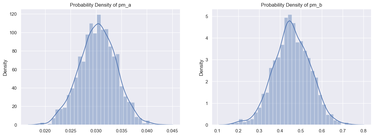
      pm_a      0.03      0.00      0.03      0.02      0.04    435.78      1.00
      pm_b      0.46      0.09      0.45      0.31      0.59    399.54      1.00

Number of divergences: 0

Code

# get param (num_samples=2000)
mcmc_samples = mcmc.get_samples()
pm_a = mcmc_samples["pm_a"]
pm_b = mcmc_samples["pm_b"]

print("mcmc_samples:", mcmc_samples)
print("pm_a:", pm_a)
print("pm_b:", pm_b)

mcmc_samples: {'pm_a': Array([0.03003247, 0.0300827 , 0.02773185, ..., 0.03265581, 0.03095045,
       0.03059688], dtype=float32), 'pm_b': Array([0.5058282 , 0.5151023 , 0.5058284 , ..., 0.37341517, 0.4465436 ,
       0.42378387], dtype=float32)}
pm_a: [0.03003247 0.0300827  0.02773185 ... 0.03265581 0.03095045 0.03059688]
pm_b: [0.5058282  0.5151023  0.5058284  ... 0.37341517 0.4465436  0.42378387]

Code

# 可視化
sns.set(style="darkgrid")
plt.figure(figsize=(15, 5))
plt.subplot(1, 2, 1)
sns.distplot(pm_a)
plt.title("Probability Density of pm_a")

plt.subplot(1, 2, 2)
sns.distplot(pm_b)
plt.title("Probability Density of pm_b")
plt.show()

C:\Users\takuk\AppData\Local\Temp\ipykernel_27764\3318693772.py:5: UserWarning: 

`distplot` is a deprecated function and will be removed in seaborn v0.14.0.

Please adapt your code to use either `displot` (a figure-level function with
similar flexibility) or `histplot` (an axes-level function for histograms).

For a guide to updating your code to use the new functions, please see
https://gist.github.com/mwaskom/de44147ed2974457ad6372750bbe5751

  sns.distplot(pm_a)
C:\Users\takuk\AppData\Local\Temp\ipykernel_27764\3318693772.py:9: UserWarning: 

`distplot` is a deprecated function and will be removed in seaborn v0.14.0.

Please adapt your code to use either `displot` (a figure-level function with
similar flexibility) or `histplot` (an axes-level function for histograms).

For a guide to updating your code to use the new functions, please see
https://gist.github.com/mwaskom/de44147ed2974457ad6372750bbe5751

  sns.distplot(pm_b)

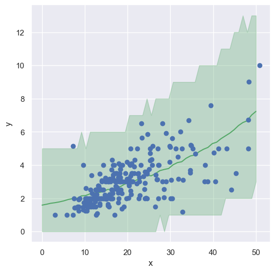
推論

Code

X_range = jnp.linspace(0, 50, 50)

predictive = Predictive(model, mcmc_samples)
predict_samples = predictive(random.PRNGKey(0), X=X_range, Y=None)
# print(predict_samples)

pm_Y = predict_samples["pm_Y"]
# print(pm_Y)

mean_Y = pm_Y.mean(axis=0)
y_low, y_high = jnp.percentile(pm_Y, jnp.array([2.5, 97.5]), axis=0)

# 可視化
fig = plt.figure(figsize=(6.0, 6.0))
plt.plot(X_range, mean_Y, "-", color="g")
plt.fill_between(X_range, y_low, y_high, color="g", alpha=0.3)
plt.plot(X, Y, "o")
plt.xlabel("x"), plt.ylabel("y")
plt.show()

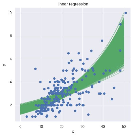
全ての推定パラメータを使って推論

Code

N = len(pm_a)
# X_range = jnp.linspace(0, 50, 50)

# 予測結果の可視化
fig = plt.figure(figsize=(6.0, 6.0))
for i in range(N):
    pm_y = [jnp.exp(pm_a[i] * x + pm_b[i]) for x in X_range]
    plt.plot(X_range, pm_y, "g-", alpha=0.5)

# データセットの可視化
plt.plot(X, Y, "o")
plt.xlabel("x"), plt.ylabel("y")
plt.title("linear regression")
plt.show()

Code

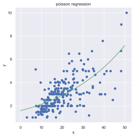
def my_model(mcmc_samples, X):
    """ポアソン回帰モデル"""
    mcmc_samples = mcmc.get_samples()
    pm_a = mcmc_samples["pm_a"]
    pm_b = mcmc_samples["pm_b"]

    # 平均値
    mu_a = jnp.mean(pm_a, axis=0)
    mu_b = jnp.mean(pm_b, axis=0)
    print("mu_a=", mu_a)
    print("mu_b=", mu_b)

    # ポアソン回帰モデル
    Y_hat = jnp.exp(mu_a * X + mu_b)

    return Y_hat


# 予測値
Y_hat = my_model(mcmc_samples, X_range)

# 可視化
fig = plt.figure(figsize=(6.0, 6.0))
plt.plot(X, Y, "o")
plt.plot(X_range, Y_hat, "g-")
plt.xlabel("x"), plt.ylabel("y")
plt.title("poisson regression")
plt.show()

mu_a= 0.030312581
mu_b= 0.45623016